Author Archives: Amy Williams

Amy Williams is a Senior Scientist at 23andMe working on the population genetics research & development team. Prior to joining 23andMe in 2022, she was an associate professor of Computational Biology at Cornell University. The opinions and tools on this website are strictly those of the author.

Estimating relationships by combining DNA from multiple siblings – DRUID

When trying to use DNA to figure out how two people are related, the closer their relationship, the easier it is. This is clear in the image below, which is from a paper that shows the rates that relatives of different degrees get classified to each of four different degrees.¹ Genetic testing companies typically don’t try to report exact degrees of relationships for relatives because, as the image shows, it’s easy to get the answer wrong (and things get even less reliable for more distant relatives than these). However, plenty of genealogists use cM sharing numbers (and the shared cM project) to try to pinpoint how two people are related.

Part of a figure from a paper that calculated the accuracy of 12 relatedness classifiers. The true relationship is given on the horizontal (in each column) and the vertical (rows) gives the detected relationship from each of the 12 tools.

This post is about a new tool called DRUID for using segments that two or more siblings share with a relative to improve the determination of their relationship. Ideally we would all test our parents’ DNA (or, if possible, their parents’ DNA), since our parents are one generation closer to our non-descendant relatives than we are.² This means that our parents are one degree of relatedness closer to our relatives, which makes for more reliable classification (as shown in the image above). If you do test your parents, consider testing their siblings as well since that gets you a larger portion of your grandparents’ DNA. The more siblings (including half-siblings) tested, the more of their parent’s DNA you have access to. On average two siblings inherit 75% of their parent’s DNA, three siblings inherit 87.5%, and |S| siblings inherit an average fraction of 1 – ½^|S| of their parent’s DNA.

Before going into the way DRUID works, the image below shows how much DRUID can improve relationship detection.³ The first row of results is for two siblings, |S| = 2; the second row is for five siblings, |S| = 5; and the columns give the true degree of relationship. The bars to compare are those of Refined IBD, which analyzes each sibling independently, and DRUID (PADRE combines information but does so differently than DRUID). As an example, for 3rd degree relatives, DRUID detects 100% of the relatives correctly compared to 80% using the method that only analyzes pairs of relatives. For 5th degree relatives, DRUID detects almost 76% correctly compared to 58.1% on average when analyzing the siblings separately.

DRUID uses the same information as Refined IBD but instead of comparing each sibling to the relative independently, it combines IBD segments from the siblings to improve accuracy. This figure is from the paper that describes DRUID.

DRUID combines segments that sibligs share with a relative to detect the parent's shared cM

DRUID merges the segments that two or more siblings share with a relative to determine how many cMs their parent shares with that person. In this image, the distant relative (black square on the right) has one blue chromosome (blue vertical bar below) and the blue regions in the sibling’s chromosomes are segments each shares with the distant relative (siblings are the black squares and circles on the bottom left, and their chromosomes are vertical bars below each shape). DRUID assumes these segments all come from one of the parents (here, the unfilled circle above the siblings; the blue regions in the vertical bars below this circle indicate the parent’s shared segments with the relative).

Briefly, the way DRUID works is that it assumes that all segments the siblings share with the relative come from only one parent and it combines those segments together (see the image on the right). It then calculates an estimate of how much of the parent’s DNA the siblings have represented using the (1 – ½^|S|) formula. DRUID assumes that this is the fraction of parent’s total cMs the siblings have inherited. So if the siblings have X cM shared with the relative, DRUID calculates T, the estimated total cM the parent shares, as T = X/F where F = 1 – ½^|S|. As the image above and several other tests from the DRUID paper show, this approach improves relationship classification.

Please don’t use DRUID if your ancestry includes endogamy or if your parents are somewhat closely related to each other. In those cases, the segments the siblings share with the relative may be a mix of DNA from both parents, and DRUID will overestimate how many cMs one parent shares with the relative.

We hope you find DRUID useful and note that the effort to get this online was a collaboration with Jonny Perl who is also launching a DRUID tool.

Thanks to Monica Ramstetter who spent many hours co-developing DRUID and calculating the accuracy of academic methods for detecting relatives (a portion of which are shown in the first image above).

IBD sharing rates across length thresholds

Some time ago, we received a request in response to our sharing rate plots for relatives with ≥ 7 cM segments to also plot rates for ≥ 5 cM segments. Instead of just calculating the rates for one more threshold, it seemed good to include several different lengths. Thus we now have a IBD sharing rates tool that allows a user to select from seven different length thresholds that range from ≥ 0 cM to ≥ 20 cM.

In other news, we have been working on extending HAPI to reconstruct the X chromosome, and the results so far are quite good! Stay tuned for updates—we will email the mailing list when this is online. (See the subscription box below.)

Thanks to Belinda Dettmann for asking about sharing rates for ≥ 5 cM segments and to Leah Larkin for asking for rates using longer segments.

Reconstructing DNA from one parent with HAPI

For RootsTech Connect this past week, we released the tool HAPI, which reconstructs DNA for one parent using data from three or more children and their other parent. Two videos from RootsTech describe ancestor DNA reconstruction in general and the HAPI tool in particular.

This post briefly reviews the video about HAPI and then goes into some technical details about it, including a few issues and questions that have come up from users in the past few days.

How much DNA can HAPI reconstruct and how accurately?

Parents transmit half of their DNA to each child, but it is a random half. One implication of this is that two siblings will have inherited different portions of their parent’s DNA, and those portions can be joined together to form more than 50% of the parent’s DNA. In fact, on average a parent transmits a fraction of 1 – ½^C of their DNA to C children. But it’s worth noting that this is just on average: sometimes the parent transmits more, sometimes less (see below).

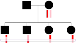
Parents transmit the same chromosome to all children at some locations.

One thing to keep in mind is that a parent transmits one DNA base pair (one “piece” of DNA) at every location to each child. So reconstructing in the way HAPI does will always get at least one copy of the parent’s two chromosome at every position (ignoring occasional errors or missing SNPs in the raw data for the children or other parent). But, as shown to the right, sometimes only one chromosome gets transmitted to all C children—here a pink colored chromosome. Therefore HAPI can only reconstruct one chromosome at some locations, and there are some technical concerns with this, as described in the next section.

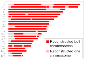
Locations where HAPI reconstructed my grandma on both or one copy.

My grandma died before genetic testing was widely available, but my dad, two aunts, one uncle, and my grandfather all consented to have their DNA tested. Using their raw data, HAPI reconstructed my grandma’s DNA, as shown on the right. For most locations, depicted in red, HAPI recovered data for both her chromosomes, but for about 10% of her DNA, HAPI recovered only one chromosome copy, as shown in pink. Overall, HAPI reconstructed 94.4% of her DNA, which is very close the average we would expect for C = 4 children, which is 93.75%, but that’s not so important—it could have been less or more.

To illustrate the variability of the amount of DNA reconstructed, we used DNA from 114 families from the San Antonio Mexican American Family Studies data (SAMAFS, analyzed here and other places) to reconstruct the father or the mother in each family, each parent in turn. The amount of reconstructed DNA in these parents varies widely, depending in part on the number of children in the family. The 114 families contain between 3 to 12 children (average 4.6), and the left plot shows the percent reconstructed in all 228 reconstructed parents (2 × 114). Focusing in on the two extremes, the top right plot gives the percent reconstructed from families with exactly 3 children, and the bottom right plot shows those with ≥ 8 children. With three children, we expect to recover 87.5% of the parent’s DNA, but in some families, we recover only 79% and in others we recover almost 92%! For large families, HAPI reconstructs nearly all of the parent’s DNA.

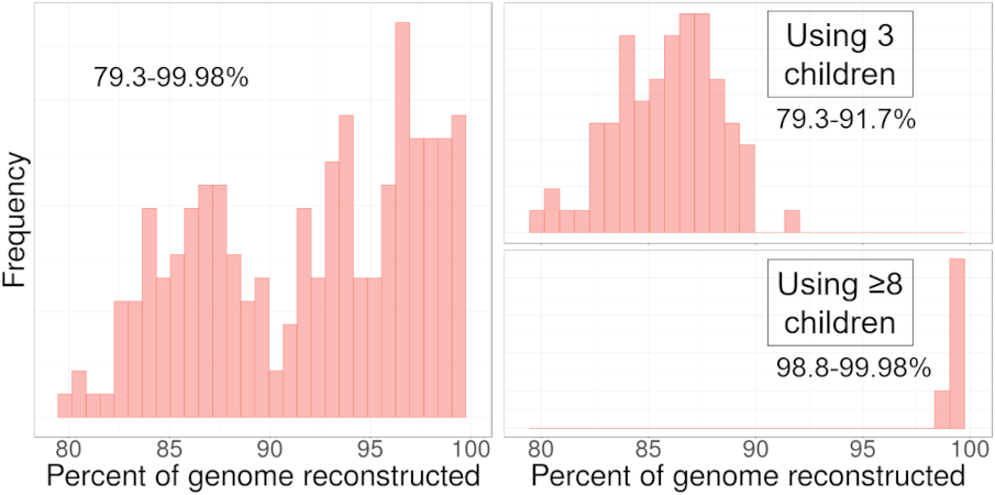
Histogram depicting the percentage of the parent’s DNA reconstructed in the SAMAFS data. Left: all families.

How accurate is the reconstructed DNA? The 114 families from the SAMAFS data actually include data from both parents, which we removed temporarily (both the father and mother in turn) to test HAPI. After running HAPI, we then compared the reconstructed DNA to the real data. The 228 reconstructed parents together have roughly 114 million SNPs, and, of those, only 36,338 differed from the truth, meaning that the reconstructed data was > 99% correct! A caveat to this is that the quality control performed on the SAMAFS data included many checks that aren’t possible to do with data from these companies, so the input data may be much more reliable than the raw data that company’s provide.

What does HAPI do in regions with only one reconstructed chromosome?

As noted above, except for cases with very large numbers of children, some portion of the parent’s DNA won’t have been transmitted and therefore there will be some parts of the genome where HAPI only recovers one of the two chromosomes. To make the printed kit readable by sites that allow uploads, HAPI currently makes two copies of the one reconstructed chromosome in those locations. So, for example, if we know that a person’s mother has an A on one chromosome, but we don’t have any information about the other chromosome, we print the SNP as being A/A. This makes the kit have “runs of homozygosity”—long regions where the person has only “homozygous” SNPs. (Homozygous SNPs are those where both of the DNA bases are the same such as C/C, and heterozygous SNPs have two bases that differ such as A/C). A drawback of this is that the parent will look inbred, but it’s not clear that a great alternative exists unless the websites that allow uploads do some engineering to allow for “half-genotyped” SNPs.

Sometime soon, we’ll allow users to select an option to print out half-missing genotypes. This will give the full information about what HAPI reconstructs, but again probably isn’t going to work for uploading to the various sites that allow uploads.

Combining different company’s raw data or different chips from the same company

Ideally all companies at all times would test people on the same set of SNPs. This would make combining data between companies or for people tested many years apart very simple. Sadly, the set of SNPs tested does vary between companies and over time for the same company. Focusing on the issue of using multiple individuals tested on different SNPs—whether from the same or different companies—a concern is that, for example, a child that is the only one that inherited, say, a red chromosome but who was not tested at a SNP that the other children were tested on can lead to a half-missing genotype in the parent. Indeed, what can happen is intermittent half-missing sites spread within a region where the parent did transmit both their chromosomes to the children. This happened in my family: my uncle was tested later than the other members of my family, has fewer SNPs than the others, and there are some places where he is the only child that inherited one of my grandma’s chromosomes. To make this more concrete, HAPI in this case may construct the following at five successive SNPs:

A/C
G/-
T/C
C/-
T/T

Interspersing “fake” full genotypes formed by repeating the one DNA base (in the above example, G at SNP 2 and C at SNP 4) to get a homozygous genotype instead of the parent’s true genotype, which may be heterozygous, can be a big problem. In general, it will lead to missed shared segments: false negatives. (If the truth is that SNP 2 is G/T and HAPI reconstructs it as G/G, that will produce a mismatch to a shared segment in a relative that does contain the T.) So, what HAPI does is, in long stretches (> 50 SNPs) of half-missing SNPs, it forms the fake runs of homozygosity, and in regions where the surrounding sites have fully reconstructed SNPs, it instead assigns what would be half-missing SNPs to be fully missing (-/-). This loss of data is less of a problem because missing genotypes—unless there are a very large number of them in a nearby location—won’t in general lead to false negative segments. Instead, the intermittent SNPs with full data will typically allow for the detection of those segments.

On the topic of using raw data from different companies, HAPI currently issues an error when a user attempts this, but there is version of the tool (linked to from the error message) that allows this. The rationale for potentially not using data from multiple companies has to do with quality control filters. Each company chooses different parameters for determining what the SNP genotypes are, and it’s possible that combining data could cause problems. However, we likely will remove this check in the future since HAPI itself detects Mendelian errors (e.g., if a parent is C/C and a child is A/A) and other forms of errors and assigns missing data to the reconstructed parent in these cases.

Other quality control filters

Related to the last section, besides detecting Mendelian and other errors, HAPI filters out SNPs where ≥ 2 individuals (the parent and/or children) are missing data. (This is increased to ≥ 3 missing SNPs when there are 6 or more children.) The reason for this is that such positions are more likely to be reconstructed as half- or fully missing and if the company determined that the SNP is missing in more than one person in a family, this is an indication that others may have erroneous data, too.

How can you use the reconstructed kit?

Several companies allow users to upload kits from other websites. This includes (alphabetically) FamilyTreeDNA, GEDmatch, Living DNA, and MyHeritage. While they may ultimately stop allowing users to upload the reconstructed data, one person wrote to say that GEDmatch accepted his HAPI reconstructed kit. Please note that this post and the availability of this tool does not indicate an endorsement of uploading these kits. Doing so may violate user agreements. However, the kits are formatted in such a way that the companies can easily prevent users from uploading them, and we hope they will not take any punitive action against users that do. (In other words, use the reconstructed kits at your own risk.)

Next steps

This version of HAPI is in “beta” (the printed kits give the current version number, 0.8b). There are several features we will add to HAPI in the near-term. One is to reconstruct the X chromosome, and, where available, Y and mitochondrial chromosomes. (SNPs on the Y and mitochondria are not provided by all companies.) Another is to produce a plot of where the parent was reconstructed on both copies and only one copy, like the one above for my grandma, and to report the percent of DNA the tool reconstructed. Also, as noted above, it will ultimately be possible to print the half-missing SNPs for positions where HAPI only reconstructed one chromosome.

Responses to questions from users

Below are a few questions people have asked.

Does Endogamy inhibit HAPI’s ability to reconstruct DNA?

The short answer is very little. The presence of one parent allows HAPI to “subtract” away that parent’s contribution to each child’s DNA. We hope to do some more analysis on this topic, but ultimately this version of HAPI (i.e., using data from one parent and multiple children) will almost certainly not attribute DNA from the parent with data to the parent being reconstructed.

What if I only have data from siblings but neither parent?

Unfortunately, unless you have, for example, ≥ 10 siblings or so, HAPI cannot to do much to help with reconstruction. The reason is that telling apart which parent is which in the data is extremely difficult. In fact, the reconstruction in large families would also have this problem, but differences in male and female recombination patterns (the subject of an upcoming blog post) allows this to work. If you’re a part of such a large family, go ahead and collect the DNA of as many of the children as you can: this tool will come!

What if I have siblings and an aunt or uncle?

Having data from an aunt or uncle would help and we can extend HAPI to work in this way. In fact, a student at Cornell is hoping to release such a tool in the near term (later this year). Once that happens, we will incorporate it onto this website, so stay tuned! (We’ll announce the release of this on our mailing list.)

What about half-siblings?

Reconstructing DNA from the shared parent of half-siblings is quite possible, and would be made even more effective if data for the non-shared parent of one or more of those half-siblings is available. While HAPI cannot yet do this—and in fact, the tool will be quite different from HAPI so will have a different name—we plan to work on this and hope to release a tool in 8-9 months. (This post is date stamped, so we’ll do our best! Again, this will be announced on the mailing list.)

What if I have a parent and two or one children?

The minimum of three children is somewhat arbitrary, and we will likely allow for the reconstruction of a parent from two children soon. Mostly, we need to do some checks to confirm that some features of HAPI work reliably in this case.

For one child, reconstruction can only provide the DNA that’s already present in that child. If someone writes with a good use case, we will likely extend to this case, but note that the reconstructed kit will be homozygous (or missing) everywhere, and may be rejected by all companies. It is not obvious how useful it will be: the matching relatives should be the same as those for the child.

Acknowledgments

This web version of HAPI extends on the original HAPI which was first written over 10 years ago. We hope to publish a paper on HAPI2 (which this website runs) later this year. For the web version, special thanks are due to Ed Williams, Debbie Kennett, and Shai Carmi who shared raw data from the various testing companies so that HAPI is able to read in data from (alphabetically) 23andMe, AncestryDNA, FamilyTreeDNA, Living DNA, and MyHeritage.

Minimal viable genetic maps

In our first blog post on what is a centiMorgan?, we talked about genetic maps. Many of the planned tools at HAPI-DNA (and all of the current ones) use genetic maps to calculate lengths of segments or to simulate segments. One of the most commonly used genetic maps (the HapMap map) contains nearly 3.4 million entries. When doing web-based analyses like those we feature here, it’s good to reduce the number of map entries. This post talks about how to drop sites from a genetic map without dramatically reducing its usefulness. Using the tool we produced for this reduces the HapMap map to just over 32,000 entries (a >100-fold reduction!). We might call this a minimal genetic map. (The title of this post is inspired by minimal viable genomes.)

Readers primarily interested in genetic genealogy may find this post a bit less useful than others. More posts about segment sharing among relatives are in the works.

Genetic maps only give a limited number of entries—not one for all >3 billion base-pairs in the human genome. Therefore, finding a genetic position for a physical position that’s not directly included in a map typically involves interpolation. A map entry lists a physical position and its corresponding genetic position, usually in centiMorgans (cM). Most IBD segments won’t have physical start and end positions listed in the map, so the standard approach is to linearly interpolate using the map positions before and after to find the genetic positions. For example, if the genetic map lists physical position 1,000,000 as being at genetic position 1.0 cM, and if the next physical position in the map is 1,200,000 at 1.2 cM, we could linearly interpolate to get the location of physical position 1,100,000. That physical position is halfway between the two flanking physical positions in the map, so its genetic position would be 1.1 cM—halfway between the two flanking genetic positions.

Cumulative distribution of a human genetic map

HapMap genetic map for human chromosome 10.

Genetic maps do not always change in a linear way between positions. This means that, if we drop entries in our genetic map arbitrarily, linear interpolation could end up giving cM positions that are far off from their true values. The image here plots the HapMap map for chromosome 10, with physical positions on the x-axis and the corresponding genetic (cM) position on the y-axis. The relationship is not linear (a zoomed in view in a smaller region would make this even more obvious), so we can’t drop positions without some care.

Instead of arbitrarily dropping map entries, the (non-web-based) tool for reducing genetic maps only drops positions where, if that location were to be linearly interpolated from the flanking locations, the difference (error) to the original map would be less than 0.05 cM. This is a tiny difference and should not meaningfully impact nearly any analysis we might want to do with IBD segments. The details of how this tool works are beyond our scope, but in general it scans a set of positions until it finds one that has minimum linear interpolation error (below 0.05 cM) and drops that entry. Following this, the tool restarts its scan to find the next entry with minimal error and drops this if it can, repeating the process until any remaining entries would produce more than 0.05 cM of error if they were linearly interpolated from their two flanking positions.

A map with only 32,143 entries, as this minimal map has, is great for the WebAssembly tools hosted on HAPI-DNA. WebAssembly tools run on the viewer’s computer—on your computer. The map is stored in only roughly 251 KB (with a four byte integer for the physical position and four byte floating point number for the cM position for each entry). The original sex-specific genetic map used for web-based simulating contains 833,777 entries, but after removing positions that can be interpolated with ≤ 0.05 cM error, it contains only 43,128 entries. With two cM positions per site—one male and one female—this map fits in 518 KB of memory.

If there is interest in comments or on Twitter, we’ll post the WebAssembly code for the segment length tool.

Thanks to Jonny Perl for collaborating on the idea of having a web-based cM calculator.

How often do two half relatives share DNA?

Following up on the last post about full relatives, the plot below shows the rates that half relatives share ≥ 7 cM IBD segments. This uses the same abbreviations as in the previous post—1C means first cousins, 3C1R stands for third cousins once removed—but all relationships are prefixed with an `h’ for half. The first relationship, hAV, is half-aunt/uncle-niece/nephew. Papers often refer to aunt/uncle and niece/nephew relatives as “avuncular,” so the plot uses AV as an abbreviation.

The rates are very similar to the “roughly” equivalent full relatives from before (see the table of equivalent relationships), but are a bit lower here. For example, half-third cousins (h3C) share at least one ≥ 7 cM segment in 71.1% of pairs versus the rate in third cousins once removed (3C1R—a roughly equivalent full relationship) of 72.7%.

Details of the simulation are the same as in the last post. This includes using the same number of pairs (100,000) for each relationship type.

Some have asked about rates for different minimum segment lengths. This is perhaps best to represent in a tool, and we’ll work on getting one up in the coming weeks.

How often do two relatives share DNA?

Close relatives like two full siblings, an aunt and nephew, or a grandparent and grandchild always share IBD segments, so they show up in testing companies’ relative matches. However, more distant relatives may not share any IBD segments. In fact, the chance that two people share DNA decreases with the distance of their relationship. This is important to remember when doing genetic genealogy: if you don’t share segments with someone that doesn’t necessarily mean you’re not related to them. As the numbers below show, even some rare second cousins (0.02% based on this analysis) may not have any detected IBD segments.

To find out the rates that relatives share segments, one option is to simulate. We did this previously (Figure 3, the SS+intf bars), but that work counted all segments, regardless of their length. Unfortunately, reliably detecting segments shorter than 6-7 cM is hard and most companies only look for 6 or 7 cM or longer segments.

Considering only 7 cM or longer segments changes the rates that relatives share DNA, as shown in the plot below. The numbers above each bar give the percent of each relative type that share at least one ≥ 7 cM segment. (Here 1C represents first cousins, 2C second cousins, etc., and NC1R represents Nth cousins once removed.) From this, we see that first cousins share five or more ≥ 7 cM segments 100% of the time, while only 0.286% of eighth cousins share such a segment (and nearly all share only one). (See below for details on how we simulated.)

You can hover over the bars to see the percentage breakdowns across segment counts.

These numbers are from simulated relatives: 100,000 pairs for each type. If the segment is present, the simulator always reports it. A caveat therefore is that, while companies report many of the ≥ 7 cM segments, they sometimes miss some. (They also sometimes report a segment that is not real, unfortunately, though in most cases a ≥ 7 cM segment will be real.) Therefore, these numbers should be used as a guide. We could—and a future blog post may—update the numbers based on probabilities of detecting segments, but a challenge is that detection rates depend on many factors, including how many SNPs were tested in the two relatives and the method the companies use to detect the segments.

Other relative types

The simulations considered a range of full cousins and full cousins once removed. It turns out, a full Nth cousin has the same shared segment properties as a full (N-1)th cousin twice removed, so the sharing rates here apply to many more types of relatives. Specific examples of equivalent relatives are shown below along with general cases. (This table doesn’t list all relative types.)

Relationship	Equivalent relationships	Roughly equivalent relationships
1C	great-aunt/uncle	half-aunt/uncle
1C1R	2nd great-aunt/uncle	half-1C
2C	1C2R	half-1C1R
2C1R	1C3R	half-2C, half-1C2R
3C	2C2R, 1C4R	half-2C1R, half-1C3R
3C1R	2C3R, 1C5R	half-3C, half-2C2R, …
4C	3C2R, 2C4R, 1C6R	half-3C1R, half-2C3R, …
4C1R	3C3R, 2C5R, 1C7R	half-4C, half-3C2R, …
NC	(N-1)C2R, (N-2)C4R, (N-3)C6R, …	half-(N-1)C1R, half-(N-2)C3R, …
NC1R	(N-1)C3R, (N-2)C5R, (N-3)C7R, …	half-NC, half-NC2R, …

Half relatives such as half-first cousins (who share one common grandparent instead of two as in full first cousins) have very slightly lower rates of sharing segments than full relatives of the roughly equivalent type. ~~If there’s enough interest (on Twitter or in the comments), we can put up another post on half-relatives.~~ Update: See the next post for rates in half relatives.

Simulation details

The numbers in the plot above are based output from the Ped-sim program where we used a sex-specific genetic map and modeled crossover interference. We found that Ped-sim very accurately captures the total segment length that real relatives share, so the numbers in the plot should be very reliable in a scenario where a company detects all ≥ 7 cM segments with no false segments. You can run Ped-sim with sex-specific maps and interference here.

Thanks to Jonny Perl for asking about sharing rates of 4C2R, which helped motivate this post.

What is a centiMorgan?

Genetic testing companies and geneticists in general use centiMorgans (cM) to measure lengths of DNA that relatives share. You may have heard that DNA contains sequences of nucleotides—adenine, cytosine, guanine, and thymine, which are abbreviated as A, C, G, and T. One natural way to measure lengths of DNA is in terms of the number of nucleotides a segment of DNA contains. This is used in many contexts and is known as a sequence’s physical length. Physical lengths are measured in units of base pairs (bp) and give the number of nucleotides a sequence contains. So, for example, “GATTACA” is 7 bp.

The human genome: Chromosomes 1 through 22 and X and Y.

To understand centiMorgans, it’s useful to have a bit of background. We all have 23 pairs of chromosomes, having inherited one set of 23 from our father and another set of 23 from our mother. These chromosomes are physically small, with all 46 contained in our bodies’ cells, but they contain all of our DNA. The length of human chromosome 1 is roughly 249 million bp, whereas chromosome 22 is about 50.8 million bp.

When it comes to heredity, perhaps the most important cell types are the germ cells: sperm and eggs. While most human cells carry 23 pairs of chromosomes, germ cells contain only one copy of each chromosome. This is so that, once these cells fuse, the resulting fertilized egg will have 23 pairs of chromosomes.

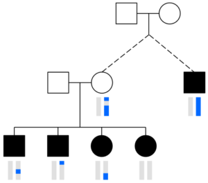
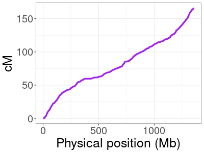
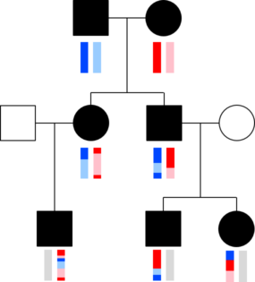
The chromosomes in germ cells are not simply an exact copy of one of the 23 chromosomes a person has, but are formed by recombination. A visualization helps capture this. The image with squares and circles shows how DNA from a couple might be transmitted to two children and three grandchildren. Here, circles represent females, squares represent males, and the vertical bars below these shapes give a colored representation of that person’s pair of chromosomes.¹ At the top, the man has a dark and a light blue chromosome, and the woman has a red and a pink chromosome. Just below them are their two children, both of whom inherited one chromosome from each parent. Because of recombination, the children’s chromosomes are multi-colored, containing copies of DNA from the their mother’s two chromosomes and from their father’s chromosomes. In this case, both children received a copy of their dad’s dark blue chromosome at the top and both also received some amount of the light blue chromosome. Similarly, the mom transmitted a chromosome to each child containing some portions from her red chromosome and some from the pink chromosome. The bars get even more colorful in the next generation—for the shapes at the bottom—because these grandchildren inherited a chromosome that is recombined from their parents’ chromosomes. This means their chromosomes can contain pieces of all four of their grandparents’ chromosomes, and indeed, copies of DNA from all four chromosomes were transmitted to at least one grandchild.

Considering all the chromosomes, a germ cell contains an average of 36.4 recombinations.² Said differently, there are an average of 36.4 recombinations per generation. In fact, this number is the Morgan length of all the chromosomes. That is, a Morgan is the average number of recombinations that occur in some piece of DNA in one generation. Of course, 36.4 Morgans is equal to 3640 cM: as its name implies, a centiMorgan is 1/100^th of a Morgan.³

Researchers have analyzed DNA from many parents and children to measure how likely a region of DNA is to recombine in one generation. They have counted not just the average number of recombinations across the full genome—i.e., 3640 cM for all the chromosomes collectively—but in specific regions, like the average on chromosome 1, or some small section of chromosome 17. A 100 cM long section of DNA (which is the same as 1 Morgan long) will have, on average, 1 recombination per generation—so a parent will usually transmit one recombination in such a section. A piece of DNA with a length of 10 cM = 0.1 Morgans has a recombination in 1 out of 10 transmissions (10%). The parent-child DNA transmission data allow researchers to produce genetic maps that anyone can use to calculate the cM length of any physical span of DNA. Genetic testing companies use these maps to calculate the length of shared segments for relatives. Perhaps the most widely used genetic map measures chromosome 1 as 286 cM and chromosome 22 is 74.1 cM. It also shows the distance from chromosome 10 physical position 34,726,104 to 83,988,506 is 49.1 cM.

In an upcoming post, we’ll talk more about cM lengths of DNA and how recombination leads more distant relatives to share fewer segments that are also on average smaller than those that close relatives share.