Category Archives: Genetic maps

In our first blog post on what is a centiMorgan?, we talked about genetic maps. Many of the planned tools at HAPI-DNA (and all of the current ones) use genetic maps to calculate lengths of segments or to simulate segments. One of the most commonly used genetic maps (the HapMap map) contains nearly 3.4 million entries. When doing web-based analyses like those we feature here, it’s good to reduce the number of map entries. This post talks about how to drop sites from a genetic map without dramatically reducing its usefulness. Using the tool we produced for this reduces the HapMap map to just over 32,000 entries (a >100-fold reduction!). We might call this a minimal genetic map. (The title of this post is inspired by minimal viable genomes.)

Readers primarily interested in genetic genealogy may find this post a bit less useful than others. More posts about segment sharing among relatives are in the works.

Genetic maps only give a limited number of entries—not one for all >3 billion base-pairs in the human genome. Therefore, finding a genetic position for a physical position that’s not directly included in a map typically involves interpolation. A map entry lists a physical position and its corresponding genetic position, usually in centiMorgans (cM). Most IBD segments won’t have physical start and end positions listed in the map, so the standard approach is to linearly interpolate using the map positions before and after to find the genetic positions. For example, if the genetic map lists physical position 1,000,000 as being at genetic position 1.0 cM, and if the next physical position in the map is 1,200,000 at 1.2 cM, we could linearly interpolate to get the location of physical position 1,100,000. That physical position is halfway between the two flanking physical positions in the map, so its genetic position would be 1.1 cM—halfway between the two flanking genetic positions.

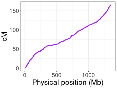
HapMap genetic map for human chromosome 10.

Genetic maps do not always change in a linear way between positions. This means that, if we drop entries in our genetic map arbitrarily, linear interpolation could end up giving cM positions that are far off from their true values. The image here plots the HapMap map for chromosome 10, with physical positions on the x-axis and the corresponding genetic (cM) position on the y-axis. The relationship is not linear (a zoomed in view in a smaller region would make this even more obvious), so we can’t drop positions without some care.

Instead of arbitrarily dropping map entries, the (non-web-based) tool for reducing genetic maps only drops positions where, if that location were to be linearly interpolated from the flanking locations, the difference (error) to the original map would be less than 0.05 cM. This is a tiny difference and should not meaningfully impact nearly any analysis we might want to do with IBD segments. The details of how this tool works are beyond our scope, but in general it scans a set of positions until it finds one that has minimum linear interpolation error (below 0.05 cM) and drops that entry. Following this, the tool restarts its scan to find the next entry with minimal error and drops this if it can, repeating the process until any remaining entries would produce more than 0.05 cM of error if they were linearly interpolated from their two flanking positions.

A map with only 32,143 entries, as this minimal map has, is great for the WebAssembly tools hosted on HAPI-DNA. WebAssembly tools run on the viewer’s computer—on your computer. The map is stored in only roughly 251 KB (with a four byte integer for the physical position and four byte floating point number for the cM position for each entry). The original sex-specific genetic map used for web-based simulating contains 833,777 entries, but after removing positions that can be interpolated with ≤ 0.05 cM error, it contains only 43,128 entries. With two cM positions per site—one male and one female—this map fits in 518 KB of memory.

If there is interest in comments or on Twitter, we’ll post the WebAssembly code for the segment length tool.

Thanks to Jonny Perl for collaborating on the idea of having a web-based cM calculator.

Genetic testing companies and geneticists in general use centiMorgans (cM) to measure lengths of DNA that relatives share. You may have heard that DNA contains sequences of nucleotides—adenine, cytosine, guanine, and thymine, which are abbreviated as A, C, G, and T. One natural way to measure lengths of DNA is in terms of the number of nucleotides a segment of DNA contains. This is used in many contexts and is known as a sequence’s physical length. Physical lengths are measured in units of base pairs (bp) and give the number of nucleotides a sequence contains. So, for example, “GATTACA” is 7 bp.

The human genome: Chromosomes 1 through 22 and X and Y.

To understand centiMorgans, it’s useful to have a bit of background. We all have 23 pairs of chromosomes, having inherited one set of 23 from our father and another set of 23 from our mother. These chromosomes are physically small, with all 46 contained in our bodies’ cells, but they contain all of our DNA. The length of human chromosome 1 is roughly 249 million bp, whereas chromosome 22 is about 50.8 million bp.

When it comes to heredity, perhaps the most important cell types are the germ cells: sperm and eggs. While most human cells carry 23 pairs of chromosomes, germ cells contain only one copy of each chromosome. This is so that, once these cells fuse, the resulting fertilized egg will have 23 pairs of chromosomes.

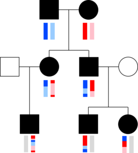
The chromosomes in germ cells are not simply an exact copy of one of the 23 chromosomes a person has, but are formed by recombination. A visualization helps capture this. The image with squares and circles shows how DNA from a couple might be transmitted to two children and three grandchildren. Here, circles represent females, squares represent males, and the vertical bars below these shapes give a colored representation of that person’s pair of chromosomes.¹For simplicity, we will talk about recombination on only one chromosome. The same principles apply to all of them—chromosome 10, 2, etc.—except the X and Y chromosomes in fathers. At the top, the man has a dark and a light blue chromosome, and the woman has a red and a pink chromosome. Just below them are their two children, both of whom inherited one chromosome from each parent. Because of recombination, the children’s chromosomes are multi-colored, containing copies of DNA from the their mother’s two chromosomes and from their father’s chromosomes. In this case, both children received a copy of their dad’s dark blue chromosome at the top and both also received some amount of the light blue chromosome. Similarly, the mom transmitted a chromosome to each child containing some portions from her red chromosome and some from the pink chromosome. The bars get even more colorful in the next generation—for the shapes at the bottom—because these grandchildren inherited a chromosome that is recombined from their parents’ chromosomes. This means their chromosomes can contain pieces of all four of their grandparents’ chromosomes, and indeed, copies of DNA from all four chromosomes were transmitted to at least one grandchild.

Considering all the chromosomes, a germ cell contains an average of 36.4 recombinations.²Technically, we should use the word crossover here. Strictly speaking, recombinations include both crossovers and another very small (10-100s of bp) form of recombination. We will follow this more typical use and say “recombination.” Said differently, there are an average of 36.4 recombinations per generation. In fact, this number is the Morgan length of all the chromosomes. That is, a Morgan is the average number of recombinations that occur in some piece of DNA in one generation. Of course, 36.4 Morgans is equal to 3640 cM: as its name implies, a centiMorgan is 1/100^th of a Morgan.³Morgans are named for Thomas Hunt Morgan who led pioneering work in the study of recombination.

Researchers have analyzed DNA from many parents and children to measure how likely a region of DNA is to recombine in one generation. They have counted not just the average number of recombinations across the full genome—i.e., 3640 cM for all the chromosomes collectively—but in specific regions, like the average on chromosome 1, or some small section of chromosome 17. A 100 cM long section of DNA (which is the same as 1 Morgan long) will have, on average, 1 recombination per generation—so a parent will usually transmit one recombination in such a section. A piece of DNA with a length of 10 cM = 0.1 Morgans has a recombination in 1 out of 10 transmissions (10%). The parent-child DNA transmission data allow researchers to produce genetic maps that anyone can use to calculate the cM length of any physical span of DNA. Genetic testing companies use these maps to calculate the length of shared segments for relatives. Perhaps the most widely used genetic map measures chromosome 1 as 286 cM and chromosome 22 is 74.1 cM. It also shows the distance from chromosome 10 physical position 34,726,104 to 83,988,506 is 49.1 cM.

In an upcoming post, we’ll talk more about cM lengths of DNA and how recombination leads more distant relatives to share fewer segments that are also on average smaller than those that close relatives share.